Zirconia Ceramics,Zirconia Engineering Components,Zirconia Precision Parts,Zirconia Wear Resistant Parts Yixing Guanming Special Ceramic Technology Co., Ltd , https://www.guanmingceramic.com
Detailed analysis of convolutional layer, TensorFlow and overall CNN structure
In the last century, scientists uncovered several visual neurological characteristics. The optic nerve has a local receptive field, meaning it can detect specific regions of an image. The recognition of a complete picture is achieved through multiple localized recognition points. Different neurons are capable of identifying distinct shapes, and the optic nerve possesses a superposition ability. Images can be constructed from low-level simple lines. Later, researchers discovered that the process of concatenation mirrors the way the optic nerve processes information. In 1998, LeCun introduced LeNet-5, which significantly improved recognition performance.
This article focuses on the convolutional layer, the pooling layer, and the overall CNN architecture.
**Convolutional Layer**
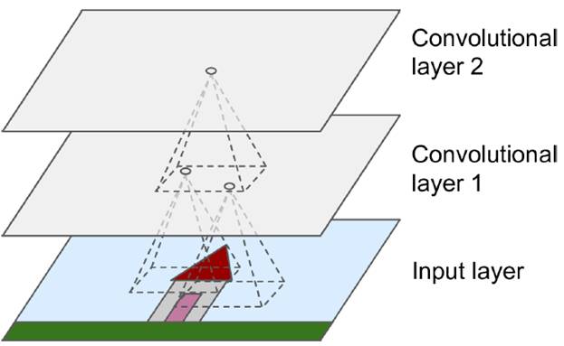
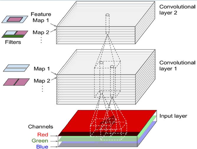
The convolutional layer mimics the concept of a local receptive field. Unlike fully connected layers, it uses small blocks of connections, known as receptive fields. By constructing specialized convolutional neurons, different responses to various shapes can be simulated. As shown in the figure below, one neuron processing a layer generates a feature map. When multiple layers are stacked, the depth increases gradually.
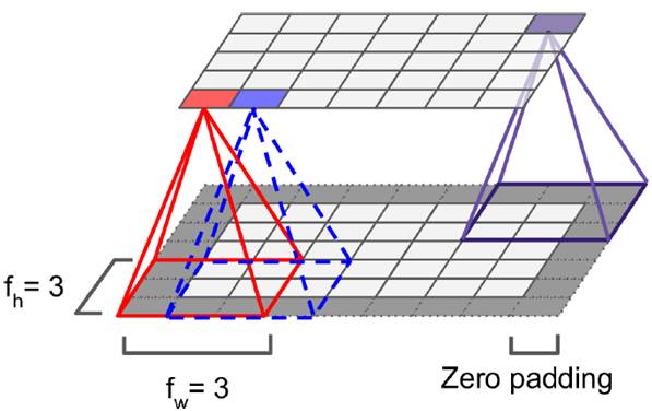
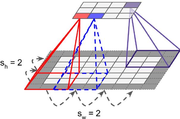
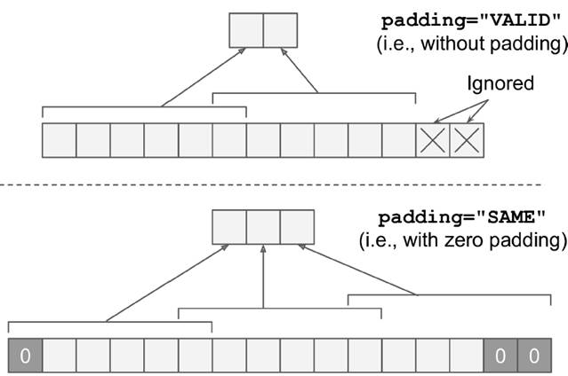
The size of the receptive field (also called kernel or filter) is denoted as fh × fw. Since the receptive field itself has a size, the feature map tends to shrink. To maintain the same size across layers, zero padding is often applied. This ensures that the output feature map remains the same size as the input. The convolution operation between layers involves multiplying corresponding pixel values. The left image shows how padding keeps the edge intact, while the right image illustrates the convolution without padding.
Although the above example is simplified, real-world images are typically three-dimensional (RGB). Instead of a matrix, they are represented as a cube. The scanning process involves a 3D block, following the same principle as in the previous examples.
Sometimes, instead of a continuous scan, the filter moves by a few pixels each time (known as stride). This reduces the feature map size compared to the original image, helping to gather important features without losing critical information.
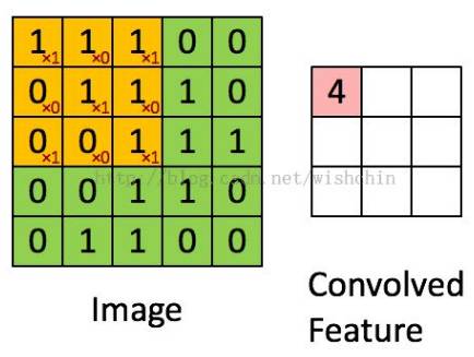
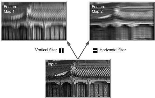
As shown in the grayscale image below, vertical and horizontal filters extract different features. Multiple such filters can be combined to create various feature maps, capturing edges, corners, and other patterns.
For RGB images, each filter scans through the 3D volume, generating a feature map. Multiple filters can stack together to form a deeper feature representation. Each pixel in the next layer is derived from a convolution operation with the previous layer's filters.
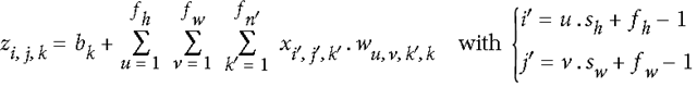
As illustrated, an output pixel value at position i-line j-column k-depth is calculated using the corresponding filter weights, input values, and bias. The formula reflects the convolution operation in detail.
**TensorFlow Implementation**
Below is an example of implementing a convolutional layer using TensorFlow:
```python
import numpy as np
from sklearn.datasets import load_sample_images
# Load sample images
dataset = np.array(load_sample_images().images, dtype=np.float32)
# Dimensions: batch_size, height, width, channels
batch_size, height, width, channels = dataset.shape
# Define 2 filters
filters_test = np.zeros(shape=(7, 7, channels, 2), dtype=np.float32)
# First filter: vertical line
filters_test[:, 3, :, 0] = 1
# Second filter: horizontal line
filters_test[3, :, :, 1] = 1
# Create a convolutional layer
X = tf.placeholder(tf.float32, shape=(None, height, width, channels))
convolution = tf.nn.conv2d(X, filters_test, strides=[1, 2, 2, 1], padding="SAME")
with tf.Session() as sess:
output = sess.run(convolution, feed_dict={X: dataset})
```
The difference between `padding="SAME"` and `padding="VALID"` is crucial. `SAME` adds zero padding to ensure all image data is included, while `VALID` only includes the parts that fit exactly.
**Memory Calculation**
Compared to fully connected layers, convolutional layers are partially connected, saving significant memory. For instance, a 5×5 filter producing 200 feature maps of 150×100 size (stride=1, padding=SAME) with an input of 150×100 RGB image (channel=3) results in 200*(5*5*3+1)=15,200 parameters. Using 32-bit floats, each image would occupy about 11.4 MB, and a mini-batch of 100 would require 1 GB of RAM.
Training CNNs is memory-intensive, but during inference, only the final output is needed.
**Pooling Layer**
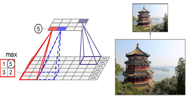
When dealing with large images, the pooling layer helps reduce memory usage by downsampling. It selects a region and represents it with a single value, either the maximum or average. A 2×2 max pooling layer with a stride of 2 compresses the image by half in both dimensions, preserving key features.
Pooling does not affect the number of channels, only the spatial dimensions.
**TensorFlow Implementation for Pooling**
```python
# Max pooling
max_pool = tf.nn.max_pool(X, ksize=[1, 2, 2, 1], strides=[1, 2, 2, 1], padding="VALID")
```
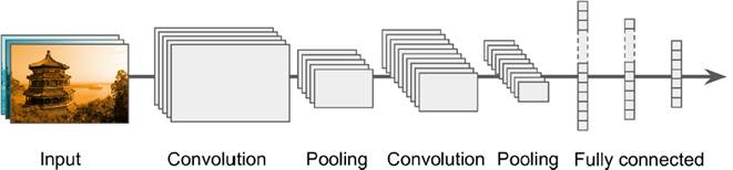
**Overall CNN Framework**
A typical CNN architecture includes convolutional and pooling layers, followed by fully connected layers. One of the earliest models was **LeNet-5**, developed in 1998. It used tanh activation functions and an RBF output layer for handwritten digit recognition.
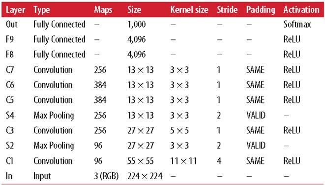
Another milestone was **AlexNet (2012)**, which introduced ReLU activation and softmax for classification, achieving over 10% improvement in accuracy.
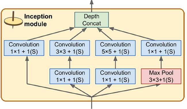
**GoogleNet (2014)** introduced the Inception module, enabling multi-scale processing and parameter efficiency through 1×1 convolutions.
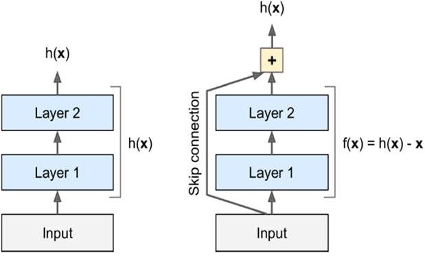
Finally, **ResNet (2015)** introduced residual learning, allowing for very deep networks by skipping layers and adding inputs directly to outputs, improving gradient flow during training.