6.560kHz
This brush is 2 In 1 Small Brush. It's a very special brush. It is small and cute. Its the aggregation with crevice nozzle and fur brush. This 2 in 1 aggregation let cleaning is more easy. You can easily remove dust edge horn corners those are difficult to clean. So people will effortlessly clean the house,they will be more happy. This brush also can be use by people to clean the computer,keyboard,sofa,bed and so on. It's a very useful brush. It also can clean the dust in the corner. It become the crevice nozzle to clean. How useful it is,hope you will like it. Now let's see the picture blow.
2 In 1 Small Brush 2 In 1 Small Brush, Folding Brush, Small Cleaning Brush, Small Hand Brush Ningbo ChinaClean Household Appliances Manufacture Co., Ltd. , https://www.chinaclean-elec.com
Dozens of filter topologies have been devised over the years, each with its own advantages. Yet engineers often rely on a small but popular subgroup of those topologies for which "cookbook" design methods are available. They choose simpler, single-op-amp filters for the less complicated lower-order designs. But when the associated cookbook approaches fail in developing a well-behaved complex filter, engineers generally turn to more complicated topologies. However, a deeper analysis of a common single-op-amp topology (the Sallen -Key filter) can lead to some interesting results if you dig below the level of cookbook formulas. 
Sign up for a free online seminar to learn how to analyze, measure, and finally solve audio system design issues (English only).
A typical filter-design process has three main stages. First, you establish the frequency range to be passed, the allowable passband ripple, etc., as determined by the system requirements. Next, you determine a transfer function (mathematical filter description) that meets the requirements, usually by choosing one of the standard types: Butterworth, Chebyshev, Bessel, Elliptical, etc. This step in the process is beyond the scope of the present article, but detailed information can be obtained from the references listed at the end .
The final step is to design and implement a circuit that provides the desired transfer function. The designer typically follows a strategy similar to the following, which is quite simple when applied to the cookbook topologies:
Factor the transfer function into second-order parts. Choose a circuit topology (or topologies) that allows each second-order function to be synthesized independently. Design each stage as an independent second-order filter. Connect the resulting second-order filters in series . A limitation common to the cookbook approaches can arise at this point. Single-op-amp filters often exhibit great sensitivity to variations in their passive-component values, and filters with high Qs (ie, most higher-order filters) are particularly sensitive . This sensitivity would not be a problem with perfect passive components, but actual components are available only in a limited number of standard values. Cookbook calculations can call for a 10.095k resistor, yet the nearest value actually available might be 10.0k.
Real-component values ​​also vary from unit to unit and in response to variations in temperature and other environmental factors. The filter's sensitivity to these component variations can cause it to deviate significantly from its desired frequency response. In many cases, the designer then turns to a more complicated filter topology. The Sallen-Key TopologyThe Sallen-Key filter (Reference 1) is among the most common single-op-amp filters. Its low-pass version (Figure 1) has these design equations: 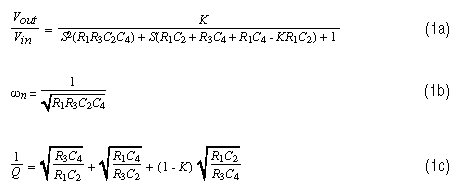 where ωn is the natural frequency, Q is the "quality factor" (a measure of the peaking that occurs near the natural frequency), and K = 1 + RB / RA is the DC gain.
Figure 1. Filter Sensitivity to Component Variations Natural-frequency and Q sensitivities are useful for evaluating transfer-function stability. For the Sallen-Key filter (given in Reference 2 on page 159), these sensitivities are as follows:  Sensitivity is represented by 'S'. Its superscript is the circuit characteristic whose sensitivity is being evaluated, and its subscript is the circuit element whose effect on that characteristic is being evaluated. Thus, the first sensitivity equation (2a) shows the sensitivity of Q to variations in R1 or R3.
S is the power to which a component variation is raised to calculate the corresponding variation in a circuit characteristic. You may have noticed, for example, that the power for all the natural-frequency sensitivities is either -1/2 or 0. When S = -1/2 and the component varies by a factor of 'A', the natural frequency varies by A-0.5 (ie, 1 / √A). Thus, the new natural frequency will be the original frequency divided by √A. When S = 0, the frequency does not change, because A0 = 1.
Reference 2 covers sensitivity in much greater detail, and it includes the derivations of many of the sensitivity equations listed above. References 3 and 4 also have good treatments of this important subject. These equations are so complicated that it often is quite difficult to choose the six passive components for a desired natural frequency and Q, while simultaneously achieving low-Q sensitivities, unless you play around with the equations and notice some interesting things that happen when the gain (K) is set to 1. K = 1 Simplifies the Sallen -Key FilterWe can simplify the Sallen-Key filter equations a great deal by choosing K = 1 as the DC gain value. In this case, the equation for Q (equation 1c) simplifies to  We also find that the sensitivity of Q to RA and RB goes to zero for K = 1 (equation 2d). This is no surprise. Setting K = 1 configures the op amp as a voltage follower by connecting its output directly to the inverting input , which eliminates RA and RB.
Substituting the simplified equation for Q (equation 3) into the sensitivity equations 2a and 2c simplifies those equations: 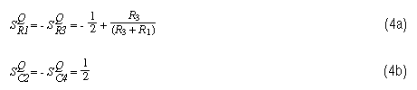 The sensitivity of Q to the resistors can be simplified further by setting the resistor values ​​equal. When R1 and R3 are exactly equal, the sensitivity is zero. But the values ​​of actual resistors are never truly equal. As they deviate from their nominal values, the sensitivity becomes non-zero but remains very small. Resistors with 5% tolerance, for example, cause a worst-case sensitivity of
 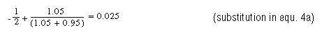 Thus, 5% resistor variations produce a 0.12% Q variation, which is negligible in comparison to the other sensitivities. Even if the resistor values ​​are not equal, this sensitivity is between -1/2 and +1/2. A closer look at the Q equation shows other reasons for setting R1 = R3:
 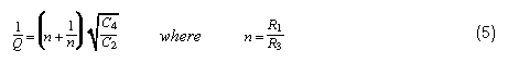 When n = 1 (ie, when R3 = R1), the quantity (n + 1 / n) has a minimum value of 2. Thus, the filter capacitors will be equal-valued when Q = 1/2 and the resistors are set equal to each other. For all Qs higher than 1/2 (the most common case by far), C2 must be larger than C4. If the resistors are not equal, the ratio of C2 to C4 must be made larger. To minimize this spread in capacitor values, the resistor values ​​should therefore be equal.
For equal resistor values, the equation for Q simplifies to 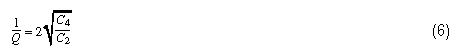 Rearranging this equation to get C2 in terms of C4,
  We can substitute this expression into the equation for
 n (equation 1b) and solve for C4:
 Substituting this result into the equation for C2 (equation 7), we get
 ![]() The Simplified Design ProcessSetting the Sallen-Key filter gain to unity and setting R1 = R3 enables the design of low-sensitivity single-op-amp filters by solving two simple equations. The simplified design process is as follows: Select an appropriate resistor value. Use equations 8 and 9 for solving the capacitor values. If C2 is too large, start over with a larger resistor value. If C4 is too small, start over with a smaller resistor value. If C4 is too small and C2 is too large, you have reached the limit for this filter. Pick standard values ​​closest to the calculated values. Two examples illustrate this method and the benefits derived from its use. Comparing the New Approach to a Cookbook ApproachThe first example comes from work done by the author several years ago. To minimize circuit variations in production, he redesigned a circuit (initially created with cookbook techniques) to realize a third-order Butterworth low-pass filter with a -3dB frequency of 4.8kHz. The redesign eli minated a trim pot and its associated need for tweaking.
The Simplified Design ProcessSetting the Sallen-Key filter gain to unity and setting R1 = R3 enables the design of low-sensitivity single-op-amp filters by solving two simple equations. The simplified design process is as follows: Select an appropriate resistor value. Use equations 8 and 9 for solving the capacitor values. If C2 is too large, start over with a larger resistor value. If C4 is too small, start over with a smaller resistor value. If C4 is too small and C2 is too large, you have reached the limit for this filter. Pick standard values ​​closest to the calculated values. Two examples illustrate this method and the benefits derived from its use. Comparing the New Approach to a Cookbook ApproachThe first example comes from work done by the author several years ago. To minimize circuit variations in production, he redesigned a circuit (initially created with cookbook techniques) to realize a third-order Butterworth low-pass filter with a -3dB frequency of 4.8kHz. The redesign eli minated a trim pot and its associated need for tweaking.
This filter required a second-order stage with Q = 1 and a natural frequency of 4.8kHz. It was implemented initially with the Sallen-Key topology and the design approach of Reference 2, pages 156 to 157, which sets the resistor values ​​equal ( R1 = R3 = R) and capacitor values ​​equal (C2 = C4 = C). Choosing C = 0.001µF resulted in gain (K) = 2 and R = 33.2K. The Q sensitivities for this circuit are as follows:  The filter was redesigned with our new method using the same resistor value (33.2kΩ). Equations 8 and 9 result in C2 = 2000pF and C4 = 500pf. The sensitivities are as follows:
  Figure 2 shows the schematics used to simulate these circuits, and Figure 3 the results of SPICE simulations. These frequency response plots are the result of a Monte Carlo run of 100 different "builds" for each filter, using 1% -tolerance resistors and 5 % capacitors. For each "build," the SPICE simulator randomly varies the component values ​​within their specified tolerances. Note that for all frequencies in the passband (especially those near the natural frequency), the new filter has substantially less variation than the old one .
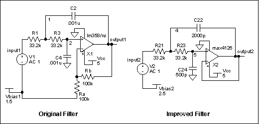
Figure 2. 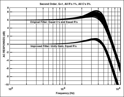
Figure 3.
It is also important to note that these simulation results are not the only steps needed to prove circuit operation; you should also build and test the circuit. Once the SPICE simulator indicates AC performance equal to that of the actual circuit with nominal component values, you can use the Monte Carlo function common in SPICE simulators to evaluate how the circuit response changes with variation in the components. Cascaded Stages Implement Higher-Order FiltersThe unity-gain Sallen-Key approach has two disadvantages. It cannot provide gain, and for high- Q filters its capacitor ratio may be too large to allow realization of the filter. Existing amplifier stages can often provide the needed gain; but, if not, the worst-case solution is to add a single-op-amp gain stage.
High-order filters often require at least one stage with a very high Q. This stage can be implemented with a more complicated topology, whereas the other stages are implemented with low-sensitivity Sallen-Key circuits. Even with Q limitations, the Sallen- Key topology can execute the high-order filters traditionally implemented with multi-op-amp topologies. The following example shows a new procedure for designing such a filter, demonstrating a dramatic improvement in performance over the older methods. Nominal specifications are as follows: Seventh -order Chebyshev 0.05dB ripple 8kHz -3dB frequency Gain = 10 An actual derivation of the transfer function from these objective specifications is beyond the scope of this article, but the references cover that subject in detail. The transfer function has three complex-pole pairs and one simple pole:
The schematics for two versions of this filter are shown in Figure 4. One was designed with the cookbook approach and the other with our new method. A single op amp in the last stage of each circuit provides the required gain and the seventh pole. 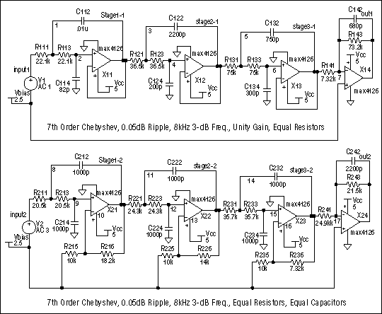
Figure 4.
Figure 5 shows the results of a Monte Carlo analysis with 1% resistors and 5% capacitors. The results are offset on the graph for visual clarity. The cookbook version has a variation of approximately 28dB near the natural frequency, rendering that design useless. In contrast, the unity-gain / equal-resistor version has a gain variation near resonance of only 4dB. 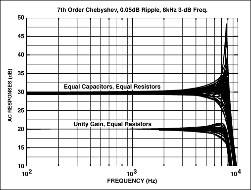
Figure 5. Sallen-Key vs. Biquad Filters It is interesting to compare this seventh-order Sallen-Key circuit with a multi-op-amp implementation of the same transfer function. The biquad is a very common three-op-amp filter that provides low sensitivity and simple design equations. Its schematic is shown in Figure 6. Using the techniques described in Reference 2, the sensitivities are as follows: 
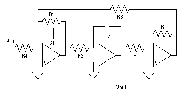
Figure 6.
The schematic for a biquad implementation of our specification is shown in Figure 7. Again, a single-op-amp stage at the end executes the gain and the seventh pole. Figure 8 compares the frequency responses for Monte Carlo analyses of the unity-gain Sallen-Key and biquad implementations (results are again offset for clarity). With equivalent components, there is no significant difference in performance between these two filters. In fact, the Sallen-Key's low-frequency gain variation is slightly smaller than that of the biquad. 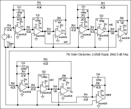
Figure 7. 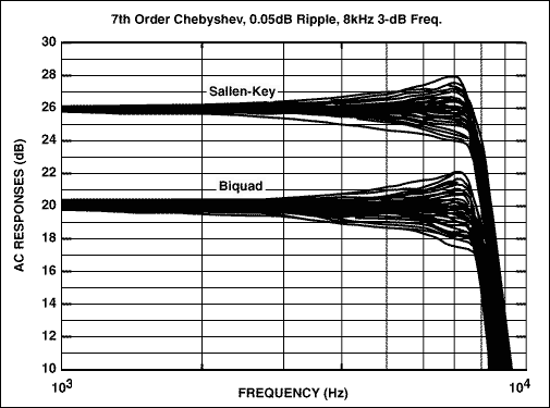
Figure 8.
The following table lists the component count, passband variation, and spread of capacitor values ​​for three implementations of the seventh-order filter just discussed:
Extending These Techniques to High-Pass FiltersWe can also design low-sensitivity high-pass filters using these techniques. The equivalent Sallen-Key high-pass filter is shown in Figure 9. Op Amps Unity Gain SK Equal R / C SK Biquad 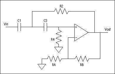
Figure 9.
Its design equations and sensitivities are as follows:  As for the low-pass case, we can simplify by setting K = 1 and (in this example) setting the capacitor values ​​equal. The equations then simplify t
  The result is two simple equations for the resistors, in which C1 = C2 = C:
 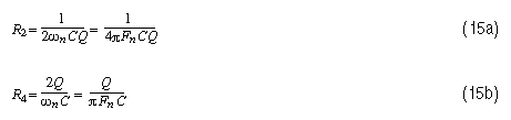 Thus, the high-pass design procedure is very similar to that of the low-pass case: Select an appropriate value for C. Calculate the resistor values ​​using equations 15a and 15b. If R4 is too large, start over with a larger C value . If R2 is too small, start over with a smaller C value. If R2 is too small and R4 is too large, then you've reached the limit for this type of filter. Pick standard values ​​closest to the calculated values. To illustrate this procedure, we can design a second-order high-pass filter stage with a Q of 1.0 and a natural frequency of 8.0kHz. First, choose C = 1200 pF. Next, set the resistor values ​​using equations 15a and 15b: R2 = 8.25kΩ and R4 = 33.2kΩ. The frequency response is plotted along with that of the low-pass filter discussed earlier (Figure 10).
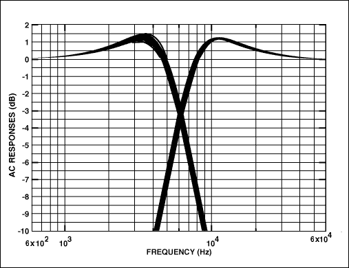
Figure 10.
The spread in frequency response for the high-pass filter is tighter than that of the low-pass filter, particularly around the peak. This occurs because we minimized sensitivity to the components with the widest variations: the capacitors. For the low-pass case , the Q sensitivity to resistors is minimized and the sensitivity to capacitors is 1/2. For the high-pass case, the sensitivity to resistors is 1/2 and the sensitivity to capacitors is minimized. We used 1% resistors and 5% capacitors , because low-tolerance resistors are more readily available than low-tolerance capacitors. If you choose 5% resistors, the two circuits exhibit a similar spread. Conclusion By delving a little more deeply into the Sallen-Key filter's component sensitivities, we found a " sweet spot "in the mathematical description that allows the design of simple, single-op-amp filters whose performance rivals that of more complicated filters. This approach has been useful in extending the utility of Sallen-Key filter s to that of higher-order higher-Q filters, and it is likely that a similar investigation into other topologies would have similar results. Appendix A Be Careful with Your Math! It is also instructive to show how the clever use of alternative mathematical representations can cause us to miss simplifications and lose sight of the physical relationships in a circuit. On page 158 of Reference 2 (the source for most of the mathematical analysis used here), the authors present a unity-gain low-pass Sallen-Key filter . They introduce the parameters m = C4 / C2 and n = R3 / R1 to simplify calculations and show the Sallen-Key Q sensitivity using these new parameters:  By not replacing Q, m, and n with their equivalent expressions in terms of resistors and capacitors, we completely miss the fact that the sensitivity to capacitors is simply 1/2. The sensitivity to resistors appears to be a function of all the capacitors and resistors, but it is actually a function of the resistors alone.
The moral of this story is that we should always substitute the actual physical quantities back into our results to check for simplifications. Appendix B Always Question Your SPICE SimulatorSchematics based on SPICE simulations of second-order filters discussed in the body of the text are shown in Figure 2. The original filter, featuring an LM358 op amp, a 5V supply, and a 1.5V virtual ground established by Vbias1, is so arranged because the LM358 cannot reliably swing closer to the positive rail than about (VCC -1.5V). With a 10% tolerance on the 5V rail, we must assume that VCC can be as low as 4.5V, so a 1.5V bias centers the signal within the minimum available range.
The new filter is built around the MAX4126, a dual op amp in the µMax package (1/2 the footprint of a standard 8-pin SO). Its input common-mode range extends beyond the rails. The output can swing to within a few millivolts of the rails when unloaded and to within 200mV when loaded with 250 Ω. This symmetrical input and output voltage range allows us to maximize the circuit's dynamic range by setting the virtual ground at VCC / 2. The combination of nearly ideal input- and output-voltage ranges also simplifies operation with a 3V power supply.
These differences in output-voltage range do not show up in the AC SPICE analyses we have run, nor are they apparent in a small-signal AC test of any real circuit, provided the op amp has sufficient bandwidth. For the same reason, these simulations give virtually identical results with most SPICE op-amp models. Only a large-signal-transient (time-domain) analysis can show the limitations on a signal range.
Good engineers always check their designs by running a transient (time-domain) analysis to ensure that they have modeled their circuits properly. They should also breadboard the circuit and take any simulation results with a grain of salt, particularly when the simulation encroaches upon signal -range limitations.
Figure 11 includes the results of two transient analyses run with TopSPICE. The first plot, which compares the MAX4126 and the LM358 output capabilities, is a simulation of the same circuit description used for AC analysis. Each output was loaded with a moderate 2kΩ load terminated at the virtual ground. 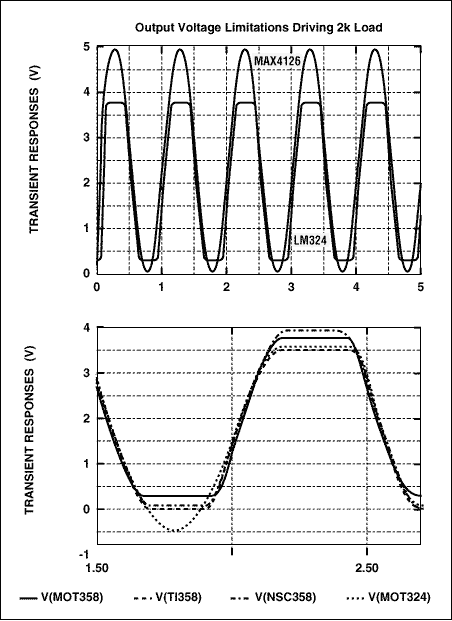
Figure 11.
The second plot shows differences among four vendor-supplied versions of the LM358 and the LM324 (a quad version of the LM358). One model indicates that the LM358 will drive all the way to ground, another shows the output going to within about 100mV of ground, and a third shows the output reaching only about 350mV. Real-circuit testing with real devices indicates that this is the more accurate result. Finally, the last model shows the output going 0.5V below the negative rail!
References Sallen, RP and Key, EL, "A Practical Method of Designing Active Filters," IRE Transactions on Circuit Theory, vol. CT-2, pp. 74 to 85, March 1955.
Huelsman, LP and Allen, PE, Introduction to the Theory and Design of Active Filters, McGraw-Hill, New York, 1980.
Budak, Aram, Passive and Active Network Analysis and Synthesis, Houghton Mifflin Company, Boston, 1974.
Ghausi, MS and Laker, KR, Modern Filter Design: Active RC and Switched Capacitor, Prentice-Hall, Englewood Cliffs, NJ, 1981.
TopSPICE mixed-mode circuit simulator, Rev 
Single Operational Amplifier Filter Minimizing Variation Sensitivity of Components-Mini
Abstract: By delving a little more deeply into the Sallen-Key filter's component sensiTIviTIes, we discover a "sweet spot" in the mathemaTIcal analysis that allows the design of simple, single op amp filters whose performance rivals that of more complicated filters. This approach has been useful in extending the uTIlity of Sallen-Key filters.
Fn
Q
7.834kHz
5.5662
1.6636
4.492kHz
0.7882
3.162kHz
simple
Circuit
Passband Variation
Resistors
Capacitors
Capacitor Spread
4dB
4
8
7
Narrow to wide
28dB
4
14
7
Narrow
4dB
10
20
7
Narrow